Environmental Sciences . 2022 September 16;3(9):1057-1064. doi: 10.37871/jbres1555.
Inference of Submerged Macrophytes Colonization Using the Weights of Evidence Method
Ligia Flávia A Batista1*, Fernanda SY Watanabe2, Luiz Henrique S Rotta2 and Nilton N Imai2
2Department of Cartography, São Paulo State University (UNESP), Rua Roberto Simonsen, 305, Presidente Prudente-SP, 19160-900, Brazil
- Spatial modeling
- Mapping
- Reservoirs
- Probabilities
Abstract
In some tropical reservoirs, aquatic macrophytes have covered extensive areas and it is difficult to monitor, control and forecast their proliferation. The major issues are economic and ecological because macrophyte growth has caused significant financial losses to hydroelectric power plants and has affected the ecological balance. Thus, this work aimed to infer the most likely areas to be colonized by Submerged Aquatic Vegetation (SAV), using influencing factors, such as the morphometric aspects of the area and any preexisting vegetation, to support the management decision-making process. Four field surveys were carried out to collect hydroacoustic data, which indicate presence of SAV, in Taquaruçu reservoir, Paranapanema River, Brazil. The inference procedure was applied using the weights of evidence method. The results showed that depths up to 6 m have a high probability of colonization and that points with five or six colonized neighbor’s cells, considering a regular grid, are also more likely to be colonized. The weights for the slope map behaved differently at each survey interval. The probability maps of colonization were generated and can be very useful in supporting the decision-making process of SAV management activities, such as concentrating the monitoring efforts for the high-probability colonization areas, in this case those which the lowest depths or next to colonized regions.
Introduction
Submerged Aquatic Vegetation (SAV) plays a key role in the ecological balance of aquatic ecosystem [1]. SAV is important to the nutrient recycling process, provides shelter to small animals, serves as a bioindicator of water quality, and contributes high quantities of organic matter to aquatic ecosystems, which is an essential process for the food chain with respect to grazing and detritus [2]. Thus, SAV represents the main component of the aquatic carbon balance [1].
The excessive colonization of water bodies by SAV is more intense in tropical areas and both ecological and economic issue has been investigated for a long time [3-5]. The economic issue is related to hydroelectric power plants, which must stop generating electricity due to turbine obstruction, causing financial losses [6-8]. In addition, other activities are hindered by SAV, such as navigation, fishing and swimming.
According to [9], some of the ecological consequences from the excessive presence of SAV are: a) an increased Biochemical Oxygen Demand (BOD) due to the decomposition of plant material; b) a reduced gas exchange rate between the aquatic environment and the atmosphere; c) interference in the primary production of phytoplankton and other trophic levels; d) the formation of an environment that is favorable to insects and mollusks that threaten sanitary conditions; and e) increased evapotranspiration.
Monitoring SAV populations is a difficult procedure and mapping techniques for this type of vegetation is aim of many studies [10-15]. Hence, it is also difficult to formulate control strategies for large Brazilian reservoirs. One of the means of sampling these populations is to use hydroacoustic survey (e.g., Sound Navigation and Ranging or Sonar). This technique uses both horizontal (area) and depth mapping to produce data and generate a bathymetric model (submerged relief) [13,16-18]. The application of this technique to SAV mapping was described by [19-21].
Using data derived by hydroacustic mapping is very important to infer how SAV colonization might expand. Such estimates can support the management decision-making process. The morphometric parameters of depth and slope, as well as the preexisting SAV, can be mapped or estimated from the bathymetric surveys, so their contribution to SAV inference can be evaluated.
Thus, the aim of this work is to map and predict the areas that are most likely to be colonized by SAV based on georeferenced data collected via hydroacoustic surveys. Such predictions are intended to identify regions with a higher probability of SAV occurrence, given the currently colonized areas and morphometric characteristics of the area. The possibility of mapping prone areas to be colonized by SAV helps the task of vegetation management, since reduce the survey fields in extensive water bodies. Thus, the main contribution of this work is to present the inference of SAV colonization, based on characteristics of the reservoir.
Study Site
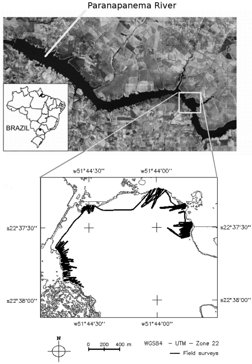
The study area is situated in the Taquaruçu reservoir, located on the Paranapanema River in the city of Santo Inácio on the border between the states of Paraná and São Paulo at the coordinates 51°44'W; 22°38'S and 51°43'W; 22°37'S. This reservoir is the second largest on the cascade of Paranapanema River and is colonized by SAV, composed mainly of the species Egeria densa and Egeria najas. The field surveys were conducted in a region of the reservoir (Figure 1) which has an area of 1.83 km2, a maximum depth of approximately 23 m, and an average depth of approximately 5 m. The flow rate of this reservoir is 18,100 m3∙s-1. The reservoir volume ranges from 179 hm3 to 210 hm3 and the water level varies from 350 m to 351 m. The hydroelectric plant has five turbines, with a total power of 525 MW. Taquaruçu reservoir is a run-of-river hydroelectric station, because it has small storage capacity, and because of this, the water coming from upstream is available for generation at that moment, and any oversupply must pass unused.
Materials and Methods
Four field surveys were performed at different time intervals in 2010 year: April 7, April 23, June 18 and August 5, to collect the hydroacoustic data. A nomenclature, composed of the‘s’ letter (survey initial) followed by a number (1 to 4) related to the survey sequence, was adopted to reference each campaign.
A digital scientific echosounder Biosonics DT-X (Biosonics, Inc., Seattle, WA, USA) was used to survey the SAV populations [22]. This model is coupled with a Global Positioning System (GPS) receiver while collecting the georeferenced data for the depth and canopy height. The echosounder is a double-frequency device that operates between 38 and 1,000 kHz frequencies to collect data up to 1,000 m depth. The echosounder is operated by a portable computer running Visual Acquisition software (BioSonics, Inc.). Post-processing was performed using the Visual Analyzer and Ecosav softwares (BioSonics, Inc., Seattle, WA, USA) for the data visualization and report generation steps, respectively. The pulse frequency adopted was 5 pps (pulses per second), and the duration of each pulse was set to 0.1 ms. Note that this equipment does not distinguish among species, only identifies the presence or absence of SAV and its canopy height. The boat speed is limited from 6 to 8 km∙h-1 to reduce the sensitivity to macrophyte flapping or swaying due to water movement. Moreover, the depth and canopy height data are generated from average measurements in a cycle or group of 10 pings, which attenuates the horizontal anomalies that could otherwise result in high errors. The regions without SAV were reported with a canopy height equal to zero; thus, every point has height information.
The studies developed by [23,24] describe how SAV can be identified from the sound pulses using the echo characteristics. Such pulses range from 40 to 60 dB in an elongated pattern. The EcoSav software has a classifying algorithm that is used to identify and distinguish SAV from the bottom depth by applying the various signal processing techniques detailed by [25].
The inset in the lower portion (Figure 1) presents the points at which the system collected the survey data. Due to the concentration of plants near shorelines, the data were acquired using a zigzag pattern, beginning from the shoreline. The boat was equipped with the system and then traveled in a perpendicular direction to the shore toward deeper areas, stopping at the vegetation limit (Figure 1). The sampling was concentrated in some parts of the reservoir where high concentration of SAV was found in surveys carried out before this experiment. Each survey lasted approximately 7 hours, because of the influence of the river current and the limited speed necessary to operate the echosounder. Because of that, and also due to the river extension, the data were collected only in a section of the reservoir.
Data Organization
The collected data were stored in a geographical database and processed using the Geographical Information System (GIS) named spring [26]. First of all, both the height of the submerged canopy and the depth of the vegetation from each survey point were imported into the GIS.
Second, the SAV map for each survey was created using Inverse Distance Weighted (IDW) interpolation and a matrix with a 2 m spatial resolution. The same method was used to produce the bathymetric model. This method is simple and can be processed faster than ordinary kriging, which was an important requisite in this work because many maps had to be interpolated. Additionally [20], considered IDW predictions are only slightly less precise than kriging; thus, such predictions were deemed appropriate for characterizing SAV in water bodies.
The surface slope angle was derived from the depth variation rate between cells, which refers to one resolution element of the regular grid. The gradient was obtained using the first- and second-order partial derivatives. The partial derivatives were calculated for each point in the depth grid using a 3 x 3 convolution window. The slope, named D, is given by Equation 9.
The Colonized Neighborhood Number (CNN) surface was also generated because the areas surrounded by the SAV are prone to colonization. This surface was produced based on the eight neighboring cells, by counting how many cells were colonized, with the zonal statistics operation available in GIS.
Spatial Inference
Spatial inference was developed for the colonization model via the weights of evidence method using the Dinamica-EGO software [27], and probability maps for particular events were generated. In this method evidence denotes the factors whose weights will be evaluated.
The weights of evidence method is used in many applications, such as mineral exploration [28], deforestation [27], urban expansion modeling [29], wildfire risk evaluation using socioeconomic data [30], both oil and gas resource assessment, landslide hazards, and the adaptability of the animal habitat [31].
This method uses the log-linear form of the Bayesian model, which is based on both a priori and a posteriori (conditional) probability concepts. It can be used when sufficient data are available to estimate the relative importance of the variable and, it is, therefore, a data-driven method [32].
The greatest advantage of this method is the possibility of combining the weights of evidence from many maps. In such case, the weights for each map can independently be calculated, given a set of spatial data, and are then combined in a sum [32].
The input maps describing the vegetation spatial distribution must be binary or multi-class. This requirement is a characteristic of the weights of evidence method. Maps with continuous numerical representations must be transformed into either binary or multi-class. Thus, in this work, the class interval is the range of values of an evidence, grouped as a class.
In this work, the heights of the submerged canopy were classified as binary data: they were denoted as ‘vegetation’ when the canopy height was greater than zero and as ‘no vegetation’ when the canopy height was equal to zero. The concept of survey interval is adopted to indicate the time, measured in days, between two consecutive field surveys. The weights of evidence were calculated by survey interval and are referred to as s1-s2, s2-s3, and s3-s4 in this text because we conducted four field surveys (i.e., s1, s2, s3, and s4).
The weights computed for each map are independent and are associated with the class interval because the raw data are continuous. Therefore, it was necessary to calculate the ranges and categorize the continuous spatial variables. These class intervals are not the same for all survey intervals because the algorithm adapts the class variables to preserve their data structure [33,34]. These breaking points are used as thresholds for the class intervals.
Other important concept of weights of evidence method is transition, which indicates the changes observed from map A for the first date and map B for the second date. Within this context, the transition is the event that changes the cells with no SAV into colonized cells, in a survey interval.
A comparison between the areas prone to colonization (the expected frequency) and the real colonization data (the observed frequency) was performed to validate these results. This procedure was performed by predicting the number of colonized cells under several characteristic combinations present in the studied area and then multiplying the conditional probability by the corresponding surface area. The predicted values were compared to observe ones to validate the results. A linear regression for each interval was applied, with the observed values placed in the ordinates (y-axis) and predicted values in the abscissas (x-axis), because the opposite regression would lead to incorrect estimates of both the slope and the y-intercept [35].
The conditional probabilities, based on depth, slope, and CNN, for each interval, were also mapped and the spatial variability was analyzed.
Results
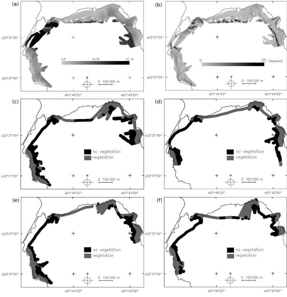
Analyzing maps for depth and slope (Figures 2a,b,e) and maps of the presence or absence of vegetation from each survey (Figures 2c-f), it is demonstrated that colonization occurs in both shallow and low-sloped areas.
The prior probabilities are given by the ratio between the colonized cells and the cells without vegetation. The transition rates are the prior probabilities divided by the survey interval, expressed in days (Table 1). As the time between survey intervals s2-s3 and s3-s4 was greater than that of s1-s2, the prior probabilities were also greater, changing from 4% for s1-s2 to 10% for both s2-s3 and s3-s4. However, when the daily transition rate is compared, the value for s1-s2 is slightly higher than the rates for the other two survey intervals. Because the daily transition rate is calculated by dividing the prior probabilities by the survey interval, the rates allow a comparison of the prior probabilities on a daily basis, without the influence of time. In this case, it can be verified that the difference between the transition rates is less significant than in the prior probability.
| Table 1: Prior probabilities and transition rates for each survey interval. | |||
| s1-s2 | s2-s3 | s3-s4 | |
| Uncolonized cells (with respect to the first survey of the interval time) | 14,587 | 13,585 | 15,439 |
| Colonized cells (the changes occurring in the transition) | 600 | 1,379 | 1,549 |
| Prior probability | 0.0411 | 0.1015 | 0.1003 |
| Survey interval (in days) | 16 | 55 | 47 |
| Transition rate (daily) | 0.0026 | 0.0019 | 0.0023 |
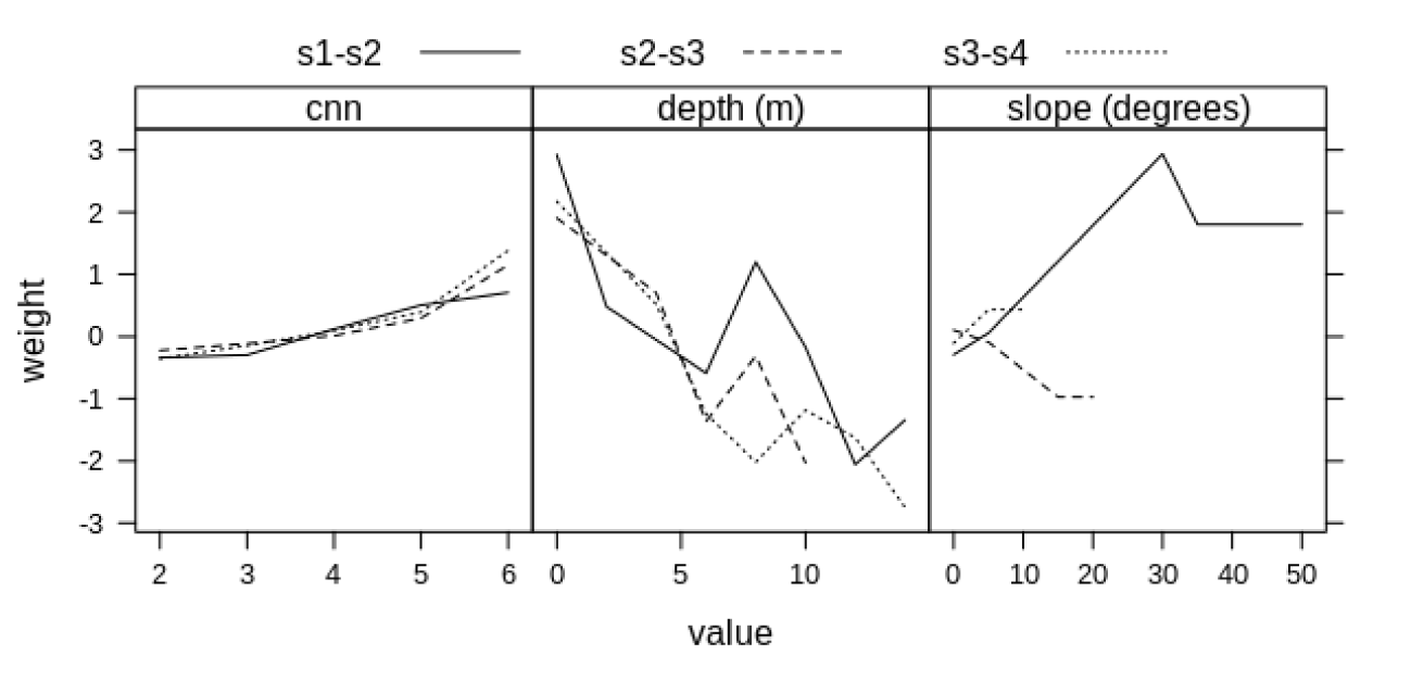
The CNN weights were very similar across the survey intervals (Figure 3). The cells with five or six colonized neighbors exhibited the greatest weights. Such finding is ecologically consistent because an area surrounded by vegetation is prone to colonization. The CNN variable was only evaluated for the uncolonized cells, for the adjacent cells to vegetation, because it characterizes the importance of a neighborhood with SAV, or preexisting population, with respect to colonization.
The depth variable with the greatest weights can be found in the first class of intervals up to a maximum depth of 6 m, for all three survey intervals. This observation suggests that colonization is favorable in these areas, possibly due to the higher light attenuation in the deeper areas. Regarding to negative weights, we can concluded that higher depth values are unfavorable to colonization, except for the 8-10 m class interval in s1-s2. This exception was likely caused by the existence of many colonization cells in this data range, which is a characteristic of empirical and data-driven method. The presence of an uncommon pattern in the data reflected in an unexpected result, which can be considered a limitation of this approach.
For the slope variable, it was possible to verify remarkable differences between the survey intervals. For s1-s2, there was a negative weight and colonization was unfavorable for the first class of intervals with a slope of up to 5°, but it was positive for class intervals of 30-35° and 35-50°. On the other hand, for the s2-s3 interval, the weight was positive, though low, for slopes up to 5° and it was negative for slopes from 15-20°. Both the s3-s4 and s1-s2 survey intervals had negative values for low slopes and positive values over the 5-10° class interval. Based on these differences we can conclude that it is not possible to determine effectively if slope interferes in colonization. For values above 20° the weights were not significant to s2-s3 survey and the same was verified above 10° for s3-s4 slope.
Regarding to the magnitude of these weights, the depth variable presented several highly positive and negative values for the different class intervals. The slope variable exhibited only one high value for the 30-35° class interval and for s1-s2. The CNN factor showed lower-magnitude weights compared to both the depth and slope. These findings indicate that the depth contributes more to the inference process than the other variables because it increases the light availability and, in this method, this also increases the conditional probability for a broader range of values than the other two variables.
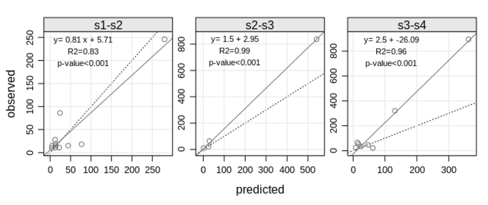
The interval s1-s2 generated the best regression between observed and predicted values for each interval (Figure 4), because the slope is closer to 1 if compared to the other intervals, although the R2 of 0.83 is smaller than 0.99 and 0.96 for s2-s3 and s3-s4, respectively.
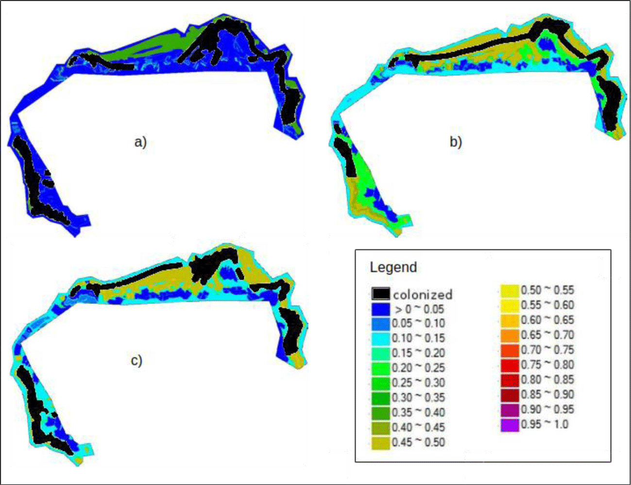
Analyzing the spatial distribution of the conditional probabilities (Figure 5), the results indicate that there is a significant difference among the survey intervals. This difference was due to the variation in weights for each survey interval regarding each indicator and the prior probabilities, which had values of approximately 0.04 for s1-s2 and 0.1 for both of the following periods (Table 1).
Generally, the pattern identified in s1-s2 shows most of the area with a probability of 0.05 as being colonized. Additionally, some regions are shown in green with a 0.4 probability of colonization.
The maps of the intervals s2-s3 and s3-s4 (Figures 5a-c) are very similar. Some differences appear because, in s2-s3 (Figure 5b), there are areas in the southwest and northeast that are uncolonized and has a 0.5 propability of containing SAV. The regions shown in the green probability class for s2-s3 (Figure 5b) have a smaller probability than that in s3-s4 (Figure 5c) because of the difference of the weights for the depth and slope.
Discussion
Of the three variables analyzed, the depth and CNN demonstrated ecologically consistent weights for the colonization dynamics, which are related to light availability and the preexisting population of the neighborhood. However, the slope variable showed both positive and negative weights, which varied significantly between the survey intervals and class intervals and are likely explained by variations in the available data. Other studies cited by [36,37] also presented different conclusions in the relationships between slope and SAV. This result suggests that the variable must be further investigated because its real influence over SAV is not completely understood.
The depth variable showed the biggest influence over the inference process based on the weights of evidence method due to the biggest weights. Other studies also have investigated the patterns of SAV in relation to depth [8,36,38,39]. This is a very useful contribution because the bathymetric map can be used to drive the monitoring task at the site [38] noted that E. densa is natively found at depths between 1 and 2 m depth and is rare in shallower or more intense water flux regions [8,36] reported that the maximum depth of SAV colonization was 7 m, which was the euphotic zone. The area within 1 m of the water margins would be considered unstable and, therefore, unfavorable to colonization, as they contain limited vertical space for growth. It also has been reported that greater depths have smaller relative growth rates due to the effects of light attenuation on photosynthesis. It is known that the euphotic depth is highly variable, even for a single location within a lake, and depends on several variables [39] presented a model of SAV height distribution from depth and water transparency measured by downwelling attenuation coefficient of Photosynthetically Active Radiation. Thus, in this work it is considered very important to evaluate whether there were meaningful contributions of depth to SAV inference.
The conditional probabilities were used to estimate the number of colonized cells and, overall, yielded good agreements for the s1-s2 interval and underestimated the number of colonized cells for the subsequent survey intervals. Thus, the estimates of the colonized areas can be considered conservative in terms of colonization, which can actually be significantly more intense.
The weights of evidence method associated with hydroacoustic mapping was considered a feasible approach for this domain because the results indicated the areas that are most prone to colonization based on the local characteristics of the water body evaluated, with an emphasis on depth. The practical implications of these findings are related to reducing the monitored area in the whole reservoir while searching for new stands of SAV. The required data to apply this method are commonly available since the morphometric variables of the area are generally known and the CNN is calculated from the SAV detected from a previous field survey. Thus, in terms of decision making method, instead of monitoring the entire length of the Taquaruçu reservoir and the Paranapanema River as a whole, the inspection could be accomplished only in the depths up to 6 m and in stands with preexisting SAV.
This approach can be reproduced in other environments, however, the weights obtained cannot be directly transferred from one environment to another. This is true for all empirical models, as in this case. In nature, empirical models which can be used in any situation are very rare or have too many parameters required to characterize the differences among each ecosystem. Thus, this type of model reaches a so high complexity level that their application may become unfeasible, as a result of the required parameters for which the data can be very scarce or difficult to measure or calibrate.
It is very hard to manage SAV because mapping alone is not sufficient when the situation is already characterized as an infestation that has become out of control. It is very important to find an efficient way of inferring or predicting the start of SAV colonization to apply the appropriate control techniques (i.e., mechanical, chemical or biological) at the beginning, to cause the least interference within the ecosystem. After an excessive colonization situation, control becomes significantly more difficult because SAV reproduce vegetatively, and, consequently, the floating fragments in the water can become rooted, transforming in other submerged canopies. All of these issues are significantly more serious if the reservoir has a large area, as is the case of many Brazilian reservoirs [40-43], where E. densa and E. najas species have been observed [8,42,44,45].
Many prediction models have been developed in the laboratory based on estimations of growth rates, taking into account the relations between biomass and various limnological variables. In these cases, the local characteristics are not considered; accordingly, these models are generic and do not represent the specific differences considered by models based on data that have been surveyed directly in situ, as proposed in this study.
Acknowledgment
The authors are grateful to the Post-graduate Program of Cartographic Sciences of São Paulo State University and to the Federal University of Technology of Paraná State for their support.
References
- Silva TSF, Costa MPF, Melack JM. Assessment of two biomass estimation methods for aquatic vegetation growing on the Amazon Floodplain. Aquat Bot. 2010;92(3):161-167. doi: 10.1016/j.aquabot.2009.10.015.
- Thomaz SM, Esteves FA. Comunidade de Macrófitas Aquáticas. [Aquatic Macrophytes Community] In: Esteves FA, editor. Fundamentos de Limnologia. Rio de Janeiro: Interciência; 2011.
- Duarte CM. Use of echosounder tracings to estimate the aboveground biomass of submerged plants in lakes. Can J Fish Aquat Sci. 1987;44(4):732-735. doi: 10.1139/f87-088.
- Duarte CM, Kalff J, Peters RH. Patterns in biomass and cover of aquatic macrophytes in Lakes: a test with Florida Lakes. Can J Fish Aquat Sci. 1988;45(11):1976-1982. doi: 10.1139/f86-235.
- Duarte CM, Kalff J. Biomass density and the relationship between submerged macrophyte biomass and plant growth form. Hydrobiologia. 1990;196(1):17-23. doi: 10.1007/BF00008889.
- Velini ED, Galo MLBT, Carvalho FT, Martins D, Cavenaghi AL, Trindade MLB, Bravin LFN, Negrisoli E, Antuniassi UR, Simionato JLA, Santos CAS. Assessment of aquatic plants in the reservoirs of AES-Tietê and development of an integrated control model for the most important species. J Environ Sci Heal. 2005;B40(1):85-101. doi: 10.1081/PFC-200034242.
- Thomaz SM, Pagioro TA, Bini LM, Murphy KJ. Effect of reservoir drawdown on biomass of three species of aquatic macrophytes in a large sub-tropical reservoir (Itaipu, Brazil). Hydrobiologia. 2006;570:53-59. doi: 10.1007/978-1-4020-5390-0_8.
- Pierini SA, Thomaz SM. Effects of limnological and morphometric factors upon Zmin, Zmax and width of Egeria spp stands in a tropical reservoir. Braz Arch Biol Technol. 2009;52(2):387-396. doi: 10.1590/S1516-89132009000200016.
- Bianchini I. Modelos de crescimento e decomposição de macrófitas aquáticas. [Growth and decomposition models of aquatic macrophytes] In: Thomaz SM, Bini M, editors. Ecologia e manejo de macrófitas aquáticas. Maringá: EDUEM; 2003. p.85-126.
- Galo MLBT, Velini ED, Trindade MLB, Santos SCA. Remote satellite sensing to monitor macrophyte dispersion in the Tietê river reservoirs. Planta Daninha. 2002;20:7-20. doi: 10.1590/S0100-83582002000400002.
- Intergraph Corporation. Intergraph Microstation PC, Version 4 User’s Guide. Bentley Systems, Inc. and Intergraph Corporation; 1991. p.333.
- Silva TSF, Costa MPF, Melack JM, Novo E. Remote sensing of aquatic vegetation: Theory and applications. Environ Monit Assess. 2008;140(1):131-145. doi: 10.1007/s10661-007-9855-3.
- Silva TSF, Costa MPF, Melack JM. Spatial and temporal variability of macrophyte cover and productivity in the eastern Amazon floodplain: A remote sensing approach. Remote Sens Environ. 2010;114(9):1998-2010. doi: 10.1016/j.rse.2010.04.007.
- Montefalcone M, Rovere A, Parravicini V, Albertelli G, Morri C, Bianchi CN. Evaluating change in seagrass meadows: A time-framed comparison of Side Scan Sonar maps. Aquat Bot. 2011;104:204-212. doi: 10.1016/j.aquabot.2011.05.009.
- Fritz C, Dörnhöfer K, Schneider T, Geist J, Oppelt N. Mapping submerged aquatic vegetation using rapideye satellite data: The example of Lake Kummerow (Germany). Water. 2017;9:510. doi: 10.3390/w9070510.
- Yadav S, Yoneda M, Susaki J, Tamura M, Ishikawa K, Yamashiki Y. A satellite-based assessment of the distribution and biomass of submerged aquatic vegetation in the optically shallow basin of Lake Biwa. Remote Sens. 2017;9:966. doi: 10.3390/rs9090966.
- Leriche A, Pasqualini V, Boudouresque CF, Bernard G, Bonhomme P, Clabaut P, Denis J. Spatial, temporal and structural variations of a Posidonia oceanica seagrass meadow facing human activities. Aquat Bot. 2006;84(4):287-293. doi: 10.1016/j.aquabot.2005.10.001.
- Sabol BM, Kannenberg J, Skogerboe JG. Integrating acoustic mapping into operational aquatic plant management: A case study in Wisconsin. J Aquat Plant Manage. 2009;47:44-52.
- Rotta LHS, Mishra DR, Watanabe FSW, Rodrigues TWP, Alcantara EH, Imai NN. Analyzing the feasibility of a space-borne sensor (SPOT-6) to estimate the height of Submerged Aquatic Vegetation (SAV) in inland waters. ISPRS J. Photogramm. Remote Sens. 2018;44:341-356. doi: 10.1016/j.isprsjprs.2018.07.011.
- Sabol BM. Innovative techniques for improved hydroacoustic bottom tracking in dense aquatic vegetation. Technical Report. Washington DC: Environmental Laboratory of U.S. Army Engineer Research and Development Center. 2001.
- Valley RD, Drake MT, Anderson CS. Evaluation of alternative interpolation techniques for the mapping of remotely-sensed submersed vegetation abundance. Aquat Bot. 2005;81(1):13-25. doi: 10.1016/j.aquabot.2004.09.002.
- Chamberlain RH, Doering PH, Orlando B, Sabol BM. Comparison of manual and hydroacoustic measurement of seagrass distribution in the Caloosahatchee estuary, Florida. Florida Scientist. 2009.
- Valley RD, Drake MT. Accuracy and precision of hydroacoustic estimates of aquatic vegetation and the repeatability of whole-lake surveys: field tests with a commercial echosounder. Technical Report. St. Paul, MN: Minnesota; Department of Natural Resources. 2005.
- Sabol BM, Melton RE, Chamberlain R, Doering P, Haunert K. Evaluation of a digital echo sounder system for detection of submersed aquatic vegetation. Estuaries Coasts. 2002;25(1):133-141. doi: 10.1007/BF02696057.
- Zhu B, Fitzgerald DG, Hoskins SB, Rudstam LG, Mayer CM, Mills EL. Quantification of historical changes of submerged aquatic vegetation cover in two bays of Lake Ontario with three complementary methods. J Great Lakes Res. 2007;33(1):122-135. doi: 10.3394/0380-1330(2007)33[122:QOHCOS]2.0.CO;2.
- Biosonics. User Guide: EcoSAV 1; Biosonics Inc: Seattle, WD, USA; 2008. p.1-48.
- Câmara G, Souza RCM, Freitas UM, Garrido J. SPRING: Integrating remote sensingand GIS by object-oriented data modelling. Comput. Gr. 1996;20(3):395-403. doi: 10.1016/0097-8493(96)00008-8.
- Soares-Filho B, Cerqueira G, Pennachin C. DINAMICA-A stochastic cellular automata model designed to simulate the landscape dynamics in an Amazonian colonization frontier. Ecol model 2002;154:217-235. doi: 10.1016/S0304-3800(02)00059-5.
- Ziaii M, Carranza EJM, Ziaei M. Application of geochemical zonality coefficients in mineral prospectivity mapping. Comput. Geosci. 2011;37(12):1935-1945. doi: 10.1016/j.cageo.2011.05.009.
- Thapa RB, Murayama Y. Urban growth modeling of Kathmandu metropolitan region, Nepal. Comput Environ Urban Syst. 2011;35(1):25-34. doi: 10.1016/j.compenvurbsys.2010.07.005.
- Romero-Calcerrada R, Barrio-Parra F, Millington JDA, Novillo CJ. Spatial modelling of socioeconomic data to understand patterns of human-caused wildfire ignition risk in the SW of Madrid (central Spain). Ecol Model. 2010;221(1):34-45. doi: 10.1016/j.ecolmodel.2009.08.008.
- Fan D, Cui X, Yuan D, Wang J, Yang J, Wang S. Weight of evidence method and its applications and development. 2011. 2nd International Conference on Challenges in Environmental Science and Computer Engineering (CESCE 2011), Procedia Environmental Sciences 11, Part C. 2011;1412-1418.
- Bonham-Carter GF. Geographic Information Systems for Geoscientists: Modelling with GIS. Vol. 13. Computer Methods in the Geosciences. Ontario: Pergamon; 1994.
- Soares-Filho BS. Rodrigues H, Costa W. Modeling Environmental Dynamics with Dinamica EGO. Belo Horizonte: Remote Sensing Center. Federal University of Minas Gerais. 2009.
- Intergraph Corporation. Intergraph Microstation PC, Version 4 User’s Guide. Bentley Systems, Inc. and Intergraph Corporation; 1991. p.333.
- Piñeiro G, Perelman S, Guerschman JP, Paruelo JM. How to evaluate models: Observed vs. predicted or predicted vs. observed? Ecol Model. 2008;216(3-4):316-322. doi: 10.1016/j.ecolmodel.2008.05.006.
- Carrillo Y, Guarín A, Guillot G. Biomass distribution, growth and decay of Egeria densa in a tropical high-mountain reservoir (NEUSA, Colombia). Aquat Bot. 2006;85:7-15. doi: 10.1016/j.aquabot.2006.01.006.
- Duarte CM, Kalff J. Littoral Slope as a predictor of the maximum biomass of submerged macrophyte communities. Limnol Oceanogr. 1986;31(5):1072-1080. doi: 10.4319/lo.1986.31.5.1072.
- Cook CDK, Urmi-König K. A revision of the genus Egeria (Hydrocharitaceae). Aquat Bot. 1984;19:73-96. doi: 10.1016/0304-3770(84)90009-3.
- Rotta LHS, Mishra DR, Alcantara E, Imai NN, Watanabe FSW, Rodrigues T. Kd(PAR) and a depth based model to estimate the height of submerged aquatic vegetation in an oligotrophic reservoir: A case study at Nova Avanhandava. Remote Sens. 2019;11(3):317. doi: 10.3390/rs11030317.
- Bini, LM, Thomaz SM. Prediction of Egeria najas and Egeria densa ocurrence in a large subtropical reservoir (Itaipu Reservoir, Brazil-Paraguay). Aquat Bot. 2005;83:227-238. doi: 10.1016/j.aquabot.2005.06.010.
- Bravin LFN, Velini ED, Reigotta C, Negrisoli E, Corrêa MR, Carbonari CA. Development of equipment for mechanical control of aquatic plants at the Americana reservoir in Brazil. Planta Daninha (Viçosa-MG). 2005;23(2):263-267.
- Nascimento PRF, Pereira SMB, Sampaio EVSB. Egeria densa biomass in the Paulo Afonso-Bahia hydroelectric plant. Planta Daninha. 2008;26(3):481-486. doi: 10.1590/S0100-83582008000300002.
- Sousa WTZ, Thomaz SM, Murphy KJ. Response of native Egeria najas Planch and invasive Hydrilla verticillata (L.f.) Royle to altered hydroecological regime in a subtropical river. Aquat Bot. 2010;92(1):40-48. doi: 10.1016/j.aquabot.2009.10.002.
- Rodrigues RR, Thomaz SM. Photosynthetic and growth responses of Egeria densa to photosynthetic active radiation. Aquat Bot. 2010;92(4):281-284. doi: 10.1016/j.aquabot.2010.01.009.
- Feitosa MF. Comparative analysis of diet, feeding selectivity and structure of the ichthyofauna, juveniles and small fish, in lateral lagoons of Rosana Reservoir (Paranapanema River, SP/PR). [dissertation]. Instituto de Biociências da Universidade Estadual Paulista: UNESP. 2011.
Content Alerts
SignUp to our
Content alerts.
 This work is licensed under a Creative Commons Attribution 4.0 International License.


